
As a subscription business, lifetime value is a very important metric for us, and this metric underpins a lot of spending and prioritising decisions for us at tails.com.
We think of lifetime value as made up of three main components: how long a customer will be active for (retention), how regularly they will order (frequency), and how much food and other products they will buy each time (order value). The focus of this blog post is the first component, and understanding how long we think customers will be active for.
Most applications of data science to customer retention seem to be classification models, predicting the likelihood that a customer will cancel before the next order or something similar. But for thinking about the total time a customer will remain active, this approach doesn't really help us. For our case we need a regression based approach, and at tails we use survival analysis to tackle this problem.
What is the average length of a subscription?
I have been asked this a few times at tails, and on the face of it it seems like a very simple question. But let's dig a little deeper into it.
Suppose we had 9 pets as below, with the bars indicating the time they had active subscriptions at tails:
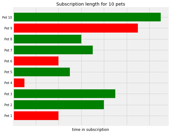
The green bars represent pets who still have an active subscription, and the red bars represent those who don't.
So to find the average subscription length of these pets, we can just take the mean of all the lengths so far, right?
Well... not quite.
As many of the pets are still active, this average will keep changing day to day and so isn't reliable. So what about just taking the average of the pets who are no longer active? Well, this will not be representative of the full pet population, particularly when we have pets who deactivated quite soon into their subscription who will be skewing the average, like Pet 4 above.
The difficulty that we have with this is because we have right-censored data. This means that for many of our data points, we haven't observed the end event, in this case when a customer is no longer active.
Survival analysis is a technique in statistics used to overcome this problem, and is used to analyse the expected time until a particular event will happen.
Survival and Hazard Functions
For a customer from our population, take T (non-negative) to be the time until this customer is no longer active. Then, the Survival Function of the population is:
$$
S(t) = \text{P}\left( T > t \right)
$$
which tells us the probability that a customer from our population is still active at time t.
Now, another statistic that we are interested in is the probability that a customer will become inactive at time t, given that they have been active up until that point. For this, we define the Hazard Function as:
$$
\lambda(t) = \lim_{h \to 0} \frac{P\left( t \le T < t + h | T \ge t\right)}{h}
$$
With a relatively simple bit of probability, you can show that the survival function and hazard function are related by:
$$
S(t) = \exp \left( - \int_{0}^{t} \lambda(s) , ds \right)
$$
The average length of a subscription, done right
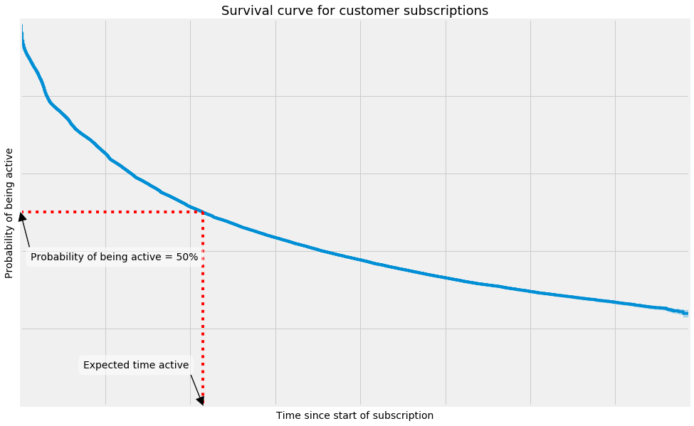
Now we take the average subscription length for our customers to be the time at which 50% of our customers have become inactive. That is, where:
$$
S(t) = 0.5
$$
In practice, we can't directly find the survival function of our population, because we have censored data. But we can estimate it using the Kaplan-Meier Estimate:
$$
\hat{S}(t) = \prod_{t_i <= t} \left( 1 - \frac{d_i}{n_i} \right)
$$
where
\begin{align}
d_i &= \text{Total churn events at time } t_i \\
n_i &= \text{Total customers at risk at time } t_i
\end{align}
which is essentially a step function where the incremental drops at each time are given by the proportion of customers who become inactive at that point.
The chart below shows how this might look for a sample of our customers:
To make all the survival curves and modelling in this blog post, I've been using the Python library Lifelines. This is a good, lightweight library with an API similar to scikit-learn libraries, and is designed to do simple survival regression, and nothing more. For this reason, it's quick and easy to pick up and start playing around with the functionality. Another great option in Python is the library scikit-survival. This library has much more functionality, and you have many more linear and non-linear model options for the modelling the survival function and hazard function.
Many books and tutorials on the subject also use examples in R, (like this one). So if you are learning this in an academic setting, then there are many great package options in R for this.
Survival Regression
What if now we group customers by different promotional campaigns that they initially came through? We see below that the survival functions for customers in different promotional groups look quite different, and so the expected time that a customer will be active is quite dependent on how you signed up in the first place:
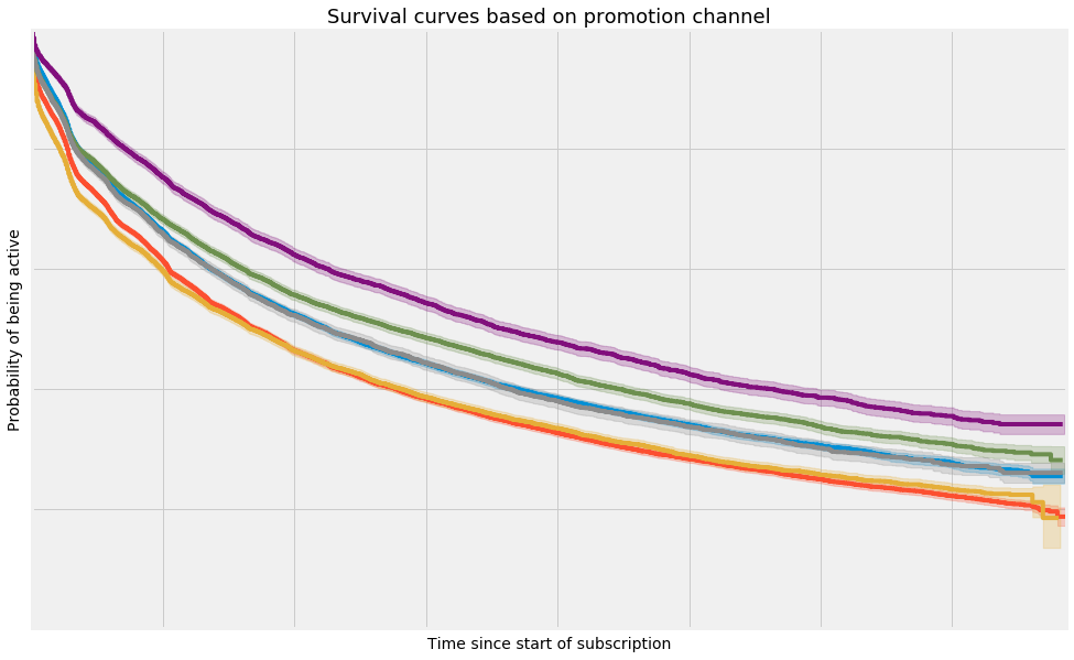
More generally, the expected time that a customer will be active depends on the customers attributes and behaviours. And to get a good estimate of how long we expect each customer to be active, we can use survival regression to find the relationship between our customer attributes and features and the survival function and hazard function of the population.
At tails, we are using survival regression to predict the time a customer will be active after their free trial, and the input data we use for this is essentially everything we know about them and their dog from the information we collect when they subscribe, and their actions during your trial, namely:
- Dog attributes: e.g. breed, allergies, previous food etc.
- Customer attributes: e.g. how you signed up, how you pay for orders etc.
- Customer actions in trial: e..g emails read, customer service contact etc.
Then we find the relationship between these features and the survival function in the population using the Cox Proportional Hazard Model. According to this model, the hazard function for the population is given by:
$$
\lambda(t) = \lambda_0(t) \exp\left(a_1 x_1 + a_2 x_2 + \dots + a_n x_n \right)
$$
for input features x.
Note that input features into this model have a multiplicative effect on the hazard function but are not time-dependent, hence the name proportional hazard. This assumption shouldn't be overlooked, and it won't hold true for all inputs that we could use into this model. There are however extensions to the Cox Proportional Hazard model that allow the impact of some features to vary with time, but I won't cover them here.
The main benefit of this model, and the reason it's so widely used in survival regression, is that the coefficients are very interpretable and give very clear insights into how the input features impact the expected time a customer will remain active for.
For our model, the feature weights for some of our factors are:
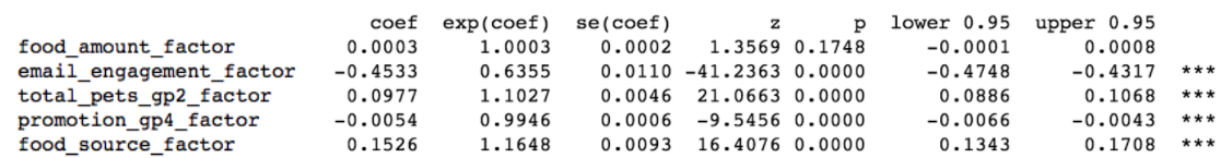
The exp(coeff) column in this summary shows you the proportional impact that each feature has on the baseline hazard function. The further this coefficient is away from 1, the greater the impact on the underlying hazard function.
Let's look at a few examples from the above output. The email_engagement_factor coefficient tells us that there is around a 36.5% decrease in the hazard of becoming inactive for somebody with an email engagement factor of 1, relative to somebody with an somebody with an email engagement factor of 0. This essentially tells us that customers who are retained for longer are more engaged with our emails. Finally, our food_amount_factor exponentiated coefficient is close to 1, and so this has a very minimal impact on the hazard function. The model is also quite unsure of what this factor should actually be. In this case, we ignore this feature in the final version of the model.
Model Accuracy - Concordance Index
Now we have a model and some nice interpretable coefficients, but how good is it exactly?
To measure the accuracy of our survival regression model, we use a Concordance Index. This is a generalisation of the AUC Score in classification models, and looks at the successful ordering of the subscription lengths of each possible pair of customers in our data. The Concordance Index is score between 0 and 1, and gives you the probability that for a randomly chosen pair of customers in our data, what is the probability that the one with a longer time active prediction will actually be active for longer.
As with the AUC, a score of 0.5 means the model is as good as random and a score of 1 means that you have a perfect predictor.
Model Output
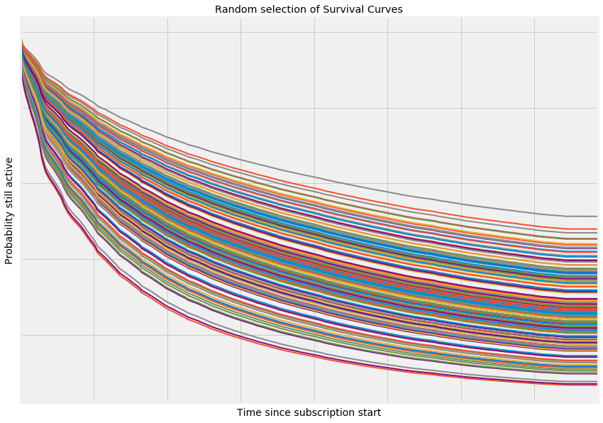
So now, let's take a quick look at the output. Below I've plotted the predicted survival functions for a random subsample of our data. You can see that there is quite a large spread between the individual survival functions for each customer. What is also clear is that none of the lines intersect. The reason for this is because of our model choice. The proportional hazards model gives a baseline hazard function which gives us the general shape of the survival curves, and then the coefficients of move the curve up or down proportionally over time.
And now we can use these predictions and the input features that are driving it to predict how long each of our customers will be active for, which will help us get a great estimate for lifetime value. And we can use this retention model directly to understand the customer segments who really love tails, and those where we can improve, so we can boost retention and get as many happy, healthy dogs in the UK feeding tails as possible.